The one-sample T-test by hand

We perform a one-Sample t-test when we want to compare a sample mean with the population mean and we do not know the population standard deviation or our sample size is small, n < 30. The difference from the Z Test is that we do not have the information on Population Variance here. We use the sample standard deviation instead of population standard deviation in this case.

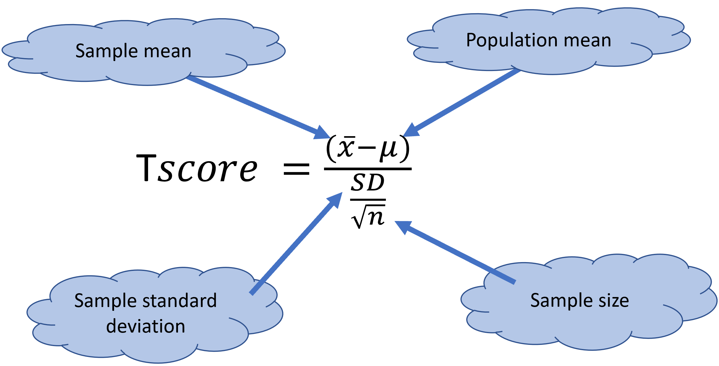
Figure 10.6: R-results for a one-sample z-test

Lets try an example.

Let’s say we want to determine if on average girls score more than 600 points in a given exam. We do not have the information related to variance (or standard deviation) for girls’ scores, so we take randomly the scores of 10 girls. We choose our \(\alpha\) value (significance level) to be 0.05.

The scores for the ten girl were:

587, 602, 627, 610, 619, 622, 605, 608, 596, 592.

Lets’ set the hypothesis

H0: \(\mu\) =< 600 the true or expected value

H1: \(\mu\) > 600 the question of interest, which in this case is to know if the girsl scored higher

In this case, we have a one-sample comparison, we do not know the population variance, and our sample size is only 10 individuals, so a T-test is best suited here.

Let’s do one by hand,

Sample=c(587, 602, 627, 610, 619, 622, 605, 608, 596, 592) #lets put the values in a vector

SampleMean=mean(Sample) #mean score of the girls sampled
SampleSD=sd(Sample) #this is the sample standard deviation
SampleSize= length(Sample)  # this is the sample size 

PopulationMean= 600 #this is the true, expected value, think of it as the population mean...

#let's now estimate the T-score using the equation above.

TTest=(SampleMean-PopulationMean)/(SampleSD/sqrt(SampleSize))
TTest

So our estimated T-value is 1.64.

Now, we need to find out the critical t-value at the 0.05 significance level. For this, we need to estimate something call Degrees of freedom, which in this case is simply our sample size minus one. In our case, the degrees of freedom, then, are 9.

With the information of the \(\alpha\) value (i.e., 0.05 in our case) and the degrees of freedom, DF (i.e, 9 in our case), we can look for the critical T-value in a table, like the one below.

Basically, scroll down the first column looking for 9 DF, then move horizontally to the column displaying the 0.05 level of significance, where they intercept that is our critical t-value. In our case that number is 1.8331.

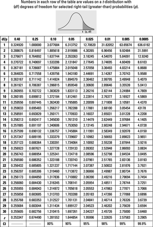
Figure 10.7: R-results for a one-sample z-test

Our critical t-value for 9DF and \(\alpha\)=0.05 is 1.8331. This means 5% of the given population are above a T-value of 1.8331.

In our case, the calculated t-value was 1.64, which is smaller than the critical value, so we fail to reject the null hypothesis and don’t have enough evidence to support the hypothesis that on average, girls score more than 600 in the exam.

There is only one T-table for cases of left-, right-, or two-tail test. When in need of a left-side score, simply remove the sign and look for the critical t-value in the table above. This is because the T-distribution is symmetric from the mean: it is the same right or left.

When in need of a two-tail test, divide the significance level by 2, and look for that value in the T-table. Say, you are using a significance level of 0.05 testing an alternative hypothesis of something being different, then you will be running a two-tail test, meaning you will be looking to see if your sample value is on either tail of the population distribution. In this case, you need to divide the significance level (\(\alpha\)) by 2 to account for the fact that you are checking the two-tails of the distribution.