The Covariance
The strength of the linear association between two variables is mathematically measured with the so-call Correlation Coefficient. The Correlation Coefficient is abbreviated with the lowercase letter \(r\) (that is not a token). However, to estimate the Correlation Coefficient, you need to first estimate the so-call Covariance.
Check a brief explanation of the covariance in the following video:
The covariance is an extension of the variance calculation we did earlier to measure the spread of the data in a variable, but in the covariance we analyze two variables. In fact, if you were to assess the relationship between a variable and itself, the covariance will be identical to the variance.
In a nutshell, the covariance tells you if the differences in two variables are trending on the same direction.
Mathematically, the covariance is calculated with the following equation:
\[\begin{equation} Covariance = COV(XY) = \frac{\sum_{i=1}^n (x -\bar{x})*(y -\bar{y})}{n-1} \end{equation}\]
Let’s try a simple example to estimate the Covariance. Let’s consider the relationship that exist between the time that you study for my class and the grade that you get.

Figure 6.3: Time stuying relates to test scores
Say, I asked five students how long they studied each week and the grade they got in my prior classes. These were the data:
| Names | Hours_Studying | Grade |
|---|---|---|
| Peter | 0.5 | 55 |
| Laura | 1.8 | 64 |
| John | 2.4 | 75 |
| Chip | 3.8 | 82 |
| Tom | 4.5 | 95 |
As always, we start by plotting the data:
StudyingTimes= data.frame(
  Names=c("Peter","Laura", "John", "Chip", "Tom"), #lets create a data.frame with three columns
  Hours_Studying=c(0.5, 1.8, 2.4, 3.8, 4.5),
  Score=c(55, 64, 75, 82,95))


#now let's do the plot
plot(Score~Hours_Studying,data=StudyingTimes,xlab="Hours a week studying", ylab="Final class score (%)")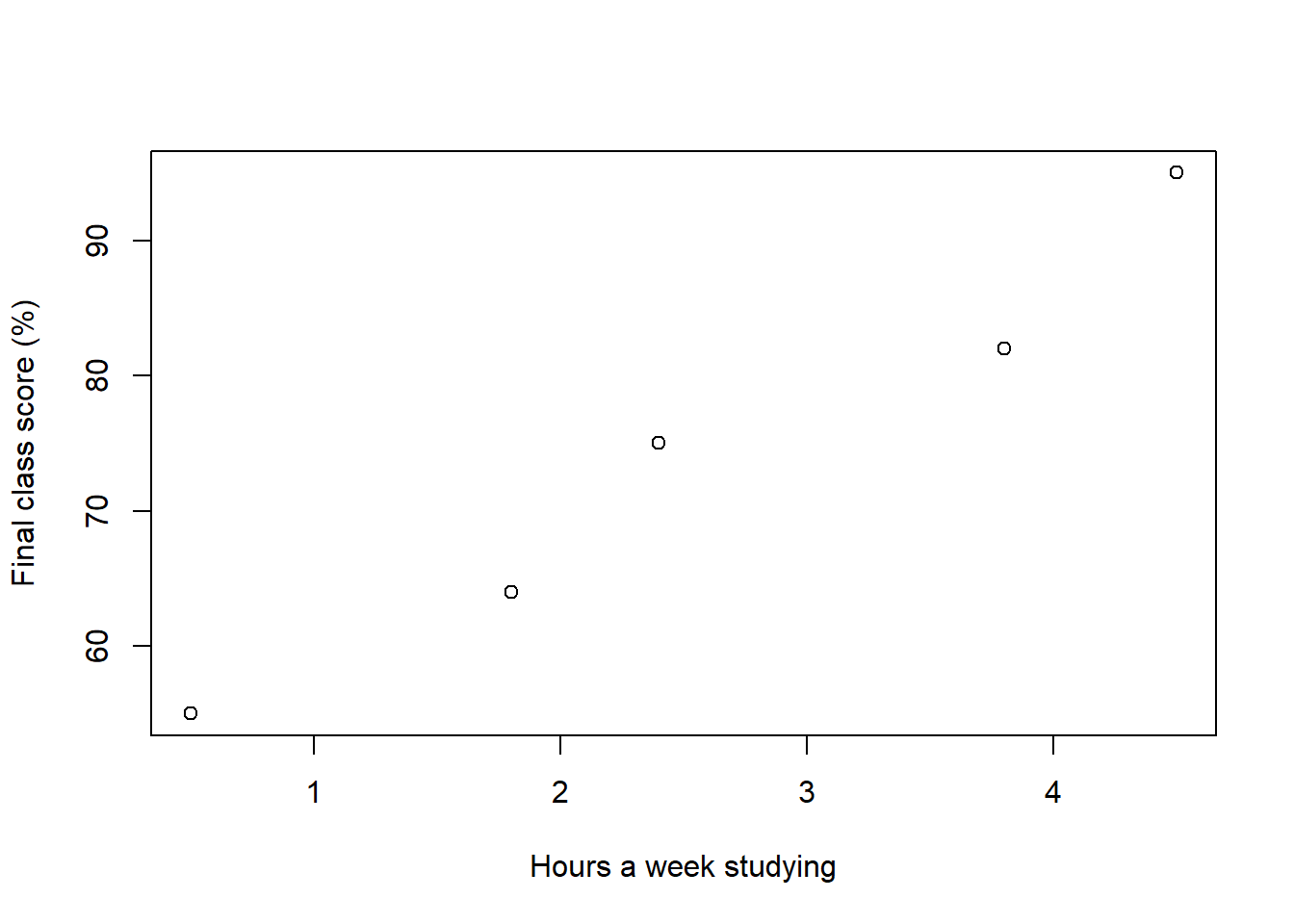
Lets break the calculation of the covariance into its parts so we can better appreciate what it does.
First, we calculate the mean of alll values in X and the difference from each value to that mean:
.png)
Figure 6.4: Differences in X
Let’s do the same for the Y-axis:
.png)
Figure 6.5: Difference in Y
Following the equation of the covariance, for the first point in the data (i.e., Peter), we place his difference to the mean in X (i.e, -2.1) and its difference to the mean in Y (-19.2), in the numerator. Like this:
.png)
Figure 6.6: Difference in X
We can do that for all data points and obtain:
\[\begin{equation} Covariance = COV(XY) =\frac{\sum_{} (-2.1)(-19.2) + (-0.8)(-10.2) + (-0.2)(0.8) + (1.2)(7.8) + (1.9)(20.8)}{5-1} \end{equation}\] . \[\begin{equation} Covariance = COV(XY) =24.3 Hours*Test Score \end{equation}\]
Hmm???, Right?…as mentioned earlier the score of the covariance by itself is hard to interpret, but it may still provide useful information about the trend of the data…in this case the covariance is positive, indicating that the differences in X trend in a positive direction as the differences in Y. Basically, as students study more they get higher grades…Please remember that!…and here it goes a token j
In R, the covariance is calculated with the cov function:
## [1] 24.3