Predict: Interpolation, Extrapolation
Ok, now we know how to build a linear regression model of the form:
\[\begin{equation} Y = mX + b \end{equation}\]
Isn’t it beauty?
That equation describes, to the best possible, how Y relates to X. With the extra support of the Coefficient of Determination, \(r^2\), you can also know how strong the relationship is.
And it just keep giving. With that relationship, you can now predict any value of Y, at any given value of X. All you have is to replace the X parameter in the equation above, for the value you like, run the calculation to get the expected value of Y.

Figure 7.7: Predictions with linear models
Let’s try. From the relationship between grades and time studying, we already know that the intercept, \(b\), was 49.28, and that the slope, \(m\), was 9.59. So, the linear model can be formulated as:
\[\begin{equation} Y = 9.59X + 49.28 \end{equation}\]
So, given that model, what would be the expected grade of a person studying 4 hours a week?. Simple, replace X for 4, run calculation and done,
\[\begin{equation} Y = 9.59* 4 + 49.28 \end{equation}\]
\[\begin{equation} Y = 87.64 \end{equation}\]
For a person that studies four hours a week the expected grade will be 87.64.
Interpolation and Extrapolation
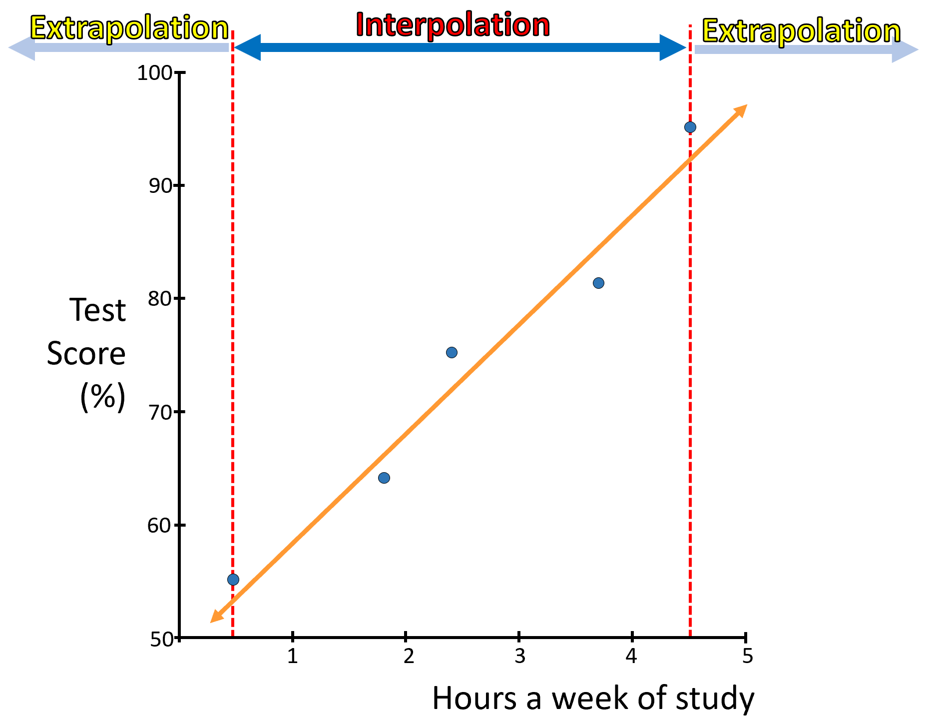
Predictions based on a linear model can be separated between those that are within the data you have, in which case the prediction is called an “interpolation”. If the prediction is beyond the values of X that you have, then the prediction is call and extrapolation.

Figure 7.8: Interpolation and Extrapolation
Needless to say, that when you extrapolate, there is always a risk that the forecast is wrong. The model you created only modeled the relationship between Y and X, for the data you have. Pass that set of data, the relationship may be different, so It is always important to be careful with extrapolations.
Predicting Y values for X values that are between observed X values in the data set is called interpolation.
Predicting Y values for X values that are beyond observed X values in the data set is called extrapolation or forecasts.In R, you can predict any value from a linear model, using the predict function, let’s try.
#take the data on grades and time studying
X=c(0.5, 1.8, 2.4, 3.8, 4.5) #hours studying
Y=c(55, 64, 75, 82,95)       #grades

# lets estimate the regression line using lm, and lets put that model in a variable
LM = lm (Y~X)   #this is the linear model between Grades~Hours_Studying

# lets now predict, the expected grades for three students that studied 1 hour, 3 hours and 10 hours
PredictGradres=data.frame(X = c(1,3,100)) #here I create a data.frame with the times studied by the three students. You need to create a column, with the same name, as the model, so lm can know which one is  the X-variable

predict(LM, PredictGradres)
## 1 2 3
## 58.86272 78.03432 1007.85680From the predictions above, you can see how the model wrongly predicts that a person that studies 100 hours a week, will get a 1000.7 grade in the class. Obviously, the most you can get is 100%. This helps to illustrate the caution needed when extrapolating a linear model beyond the limits of the data.
Two statisticians were traveling in an airplane from LA to New York.
About an hour into the flight, the pilot announced that they had lost an engine. “Don’t worry”, says the pilot, “there are three left; but, instead of 5 hours it would take 7 hours to get to New York”.
A little later, the pilot announced that a second engine failed. “Don’t worry”, says the pilot, “there are two left; but, instead of 5 hours it would take 10 hours to get to New York”.
Somewhat later, the pilot came on the intercom again and announced that a third engine had died. “Never fear”, he announced, “the plane can fly on a single engine. However, it would now take 18 hours to get to NewYork”, the pilot added.
At this point, one statistician turned to the other and said, “Gee, I hope we don’t lose that last engine, or we’ll be up here forever!”